Chapter 2　 Limit sets of Kleinian groups

Figure 2.1:

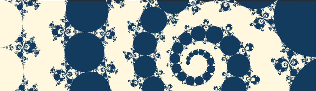
Figure 2.2:

In this chapter, we will introduce how to draw the limit set of Kleinian groups with a shader and animate the resulting fractal figure. Speaking of fractal animation, it is interesting to see a self-similar figure by scaling it up or down, but with this method, you can see a characteristic movement in which straight lines and circumferences transition more smoothly.

The sample in this chapter is "Kleinian Group" of
https://github.com/IndieVisualLab/UnityGraphicsProgramming4
.

2.1　 Yen reversal

First, I will introduce the inversion of figures. I think it is familiar that a figure that is inverted like a mirror image with a straight line as a boundary is line-symmetrical, and if it is inverted around a point, it is point-symmetrical. There is also a reversal of circles. It is an operation to switch the inside and outside of the circle on the two-dimensional plane.

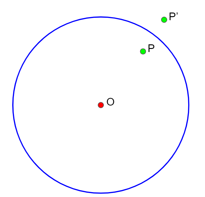
Figure 2.3: Circle Inversion P \ rightarrow P'

The center of the circle O , radius r inverted with respect to the circle of, \ Left | OP \ Right | a | '\ right | \ left OP is so as to satisfy the following equation remains the same direction P to P' to move to the operation Become.

\left| OP\right| \cdot \left| OP'\right| =r^{2}

In the vicinity of the circumference, the inside and outside appear to be interchanged like a distorted line symmetry, and the infinity far away from the circumference and the center of the circle are interchanged. What is interesting is the case where the straight line on the outside of the circle is inverted, and when it is close to the circle, it moves to the inside across the circumference and continues to infinity as it moves away from it. Become.

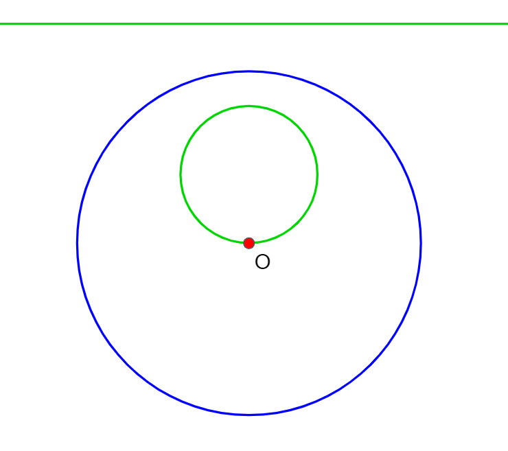
Figure 2.4: Straight line inversion

It will appear as a small circle inside the circle. If you think of a straight line as a circle with an infinite radius, you can say that circle inversion is an operation that swaps the circles inside and outside the circle.

2.1.1 Expressed by　 mathematical formula

The formula for the circle inversion of the unit circle on the complex plane is as follows.

z \ rightarrow \ dfrac {1} {\ overline {z}}

z is a complex number and \ overline {z} is its complex common benefit.

The next way and try to formula deformation z 1 divided by the square power of the length of the z you can see that is an operation that is scale.

z\rightarrow \dfrac {1}{\overline {z}}=\dfrac {1}{x-iy}=\dfrac {x+iy}{\left( x-iy\right) \left( x+iy\right) }=\dfrac {x+iy}{x^{2}+y^{2}}=\dfrac {z}{\left| z\right| ^{2}}

As a graphic operation on the complex plane,

• Sum of complex numbers: translation
• Complex product: rotation (and scaling)

I think that many people are aware that, but this is where operations including division are newly added.

2.2　 Mobius transformation

The Mobius transformation * 1 is a generalized form that includes division in the transformation on the complex plane .

z \ rightarrow \ dfrac {az + b} {cz + d}

a, b, c, d are all complex numbers.

2.3　 Schottky group, Kleinian group

Consider creating a fractal figure by repeatedly using the Mobius transformations.

Prepare four sets of circles D_A , D_a , D_B , D_b that do not intersect each other . First of which focuses on two sets of circle D_A the outside of D_a inside, D_A the inside of D_a Mobius transformation transferred to outside a create a. Similarly, make a Mobius transformation b from two other sets of circles D_B and D_b . Also , prepare the inverse transformations A and B respectively .

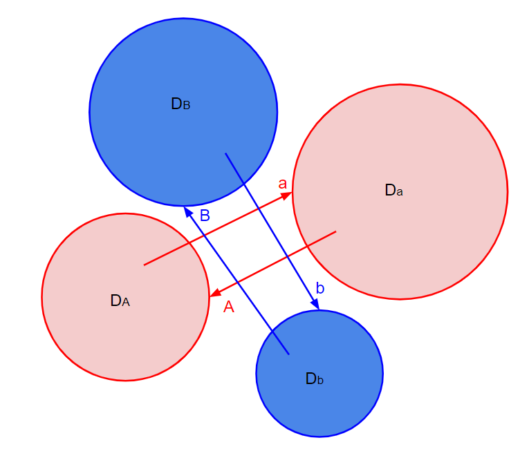
Figure 2.5:

The entire transformation (for example, aaBAbbaB ) obtained by synthesizing the four Mobius transformations a , A , b , and B in any order is called " Schottky group * 2 based on a , b ".

This is further generalized, and the discrete group consisting of Mobius transformations is called the Kleinian group . I have the impression that this name is more widely used.

2.4　 Limit set

When you display the image of the Schottky group, you will see a circle inside the circle, a circle inside it, and so on. These sets are called " the limit set of Schottky groups in a and b ". The purpose of this chapter is to draw this limit set .

2.5　 Jos Leys' algorithm

2.5.1　 Overview

I will introduce how to draw the limit set with a shader. It is difficult to implement it honestly because the combination of conversions continues infinitely, but Jos Lays has published an algorithm for this * 5, so I will try to follow it.

First, prepare two Mobius transformations.

a: z\rightarrow \dfrac {tz-i}{-iz}

b: z\rightarrow z+2

t is the complex number u + iv . The shape of the figure can be changed by changing this value as a parameter.

If you take a closer look at transformation a ,

a: z \ rightarrow \ dfrac {tz-i} {- iz} = \ dfrac {t} {- i} + \ dfrac {1} {z} = \ dfrac {1} {z} + (- v + iu )

\dfrac {1}{z}=\dfrac {1}{x+iy}=\dfrac {x-iy}{(x+iy)(x-iy)}=\dfrac {x-iy}{x^{2}+y^{2}}=\dfrac {x-iy}{\left|z\right|^{2}}

Therefore,

a: z\rightarrow \dfrac {tz-i}{-iz}=\dfrac{x-iy}{\left|z\right|^{2}}+(-v+iu)

So

1. Invert the circle in the unit circle,
2. Invert the sign of y and
3. -v + iu parallel movement

You can see that it is an operation.

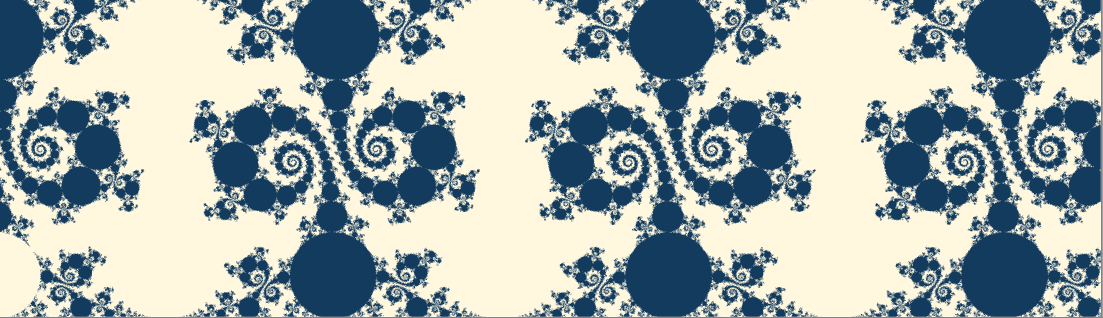
The limit set using transformations a and b and their inverse transformations is the following strip-shaped figure in which large and small circles are connected.

Figure 2.6: Limit set

Let's take a closer look at the features of this shape.

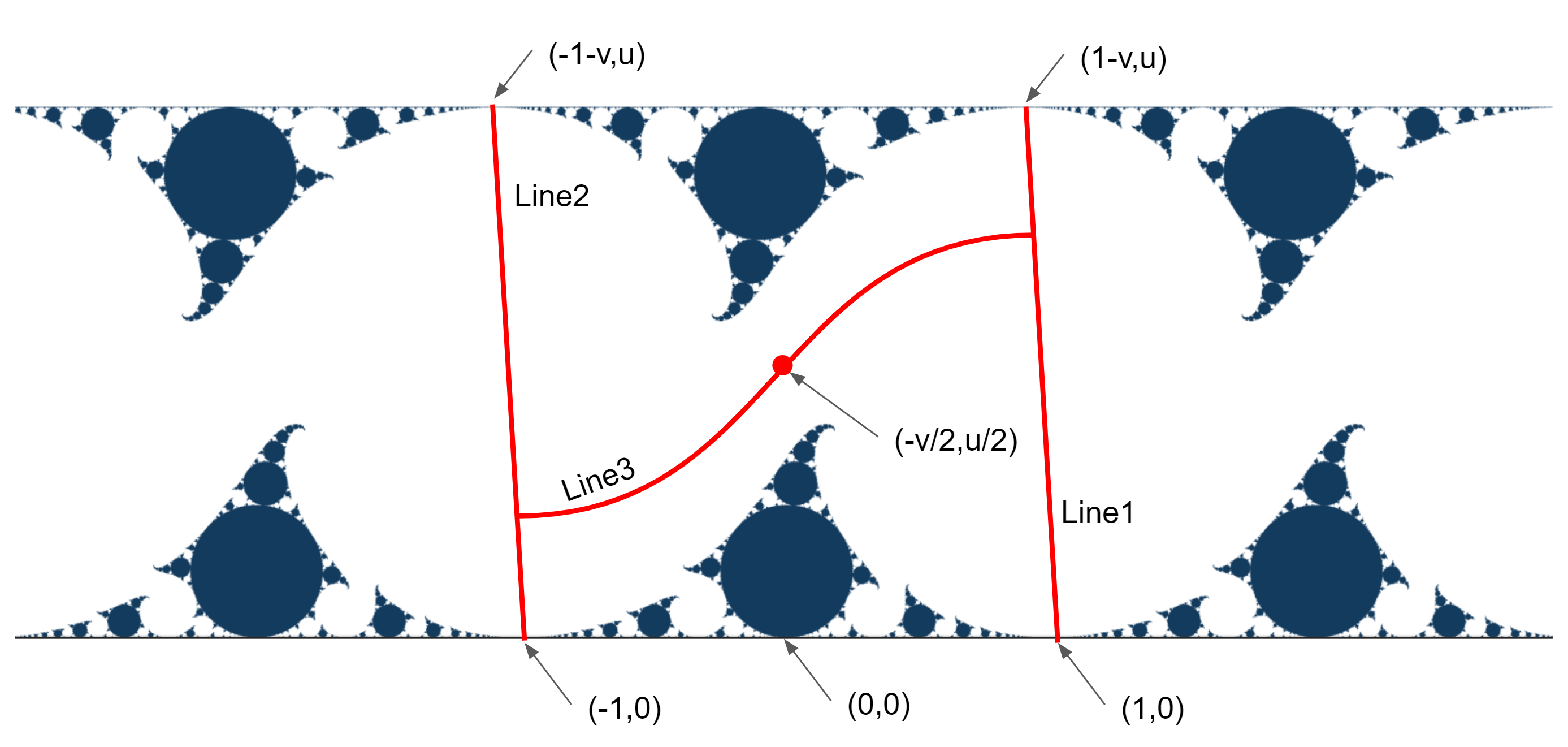
Figure 2.7:

It has a band shape of 0 \ leq y \ leq u , and the parallelograms separated by Lines 1 and 2 repeat in the left-right direction. Line1 is a straight line that passes through points (1,0) and points (1-v, u) , and Line2 is a straight line that passes through points (-1,0) and points (-1-v, u) . Line3 becomes a line that divides the figure into the upper limit, and the upper and lower figures divided by this line in the parallelogram are point symmetric at the point z =-\ dfrac {v} {2} + \ dfrac {iu} {2} It has become.

2.5.2　 Algorithm

Determines if any point is included in the limit set. Utilizing the fact that parallelogram regions repeat on the left and right, and point symmetry on the top and bottom with Line 3 as the boundary, the judgment at each point is finally brought to the judgment of the figure in the lower half of the center. ..

We will process a certain point as follows.

• If it is to the right of Line 1, move it to the left to fit within the parallelogram range
• If it's to the left of Line2, move to the right as well
• If it is above Line3, use the point symmetry and move it to the target point so that it is below Line3.
• Apply transformation a to points below Line3

The largest circle tangent to the straight line y = 0 is the inverted line y = u in the unit circle. When the conversion a is applied to the points in this, y <0 and it deviates from the band of 0 \ leq y \ leq u . Therefore,

When a point is multiplied by the transformation a , y <0 = A point is included in this largest circle = It is included in the limit set

Judgment is made as.

On the contrary, what if it is not included? Even if the above procedure is repeated, the band of 0 \ leq y \ leq u cannot be removed, and finally the movement of two points across Line 3 will be repeated. Therefore, if the points are the same as two points before, it can be judged that the points are not included in the limit set.

In summary, it will be processed as follows.

1. Out of range if y <0 , u <y
2. Move to the center parallelogram if it is to the right of Line1 and to the left of Line2
3. Invert about center point if above Line 3
4. Apply transformation a
5. If y <0, it is judged as the limit set
6. If it is the same as the previous point, it is judged that it is not the limit set
7. If neither, go back to 2.

2.6　 Implementation

Let's take a look at the code.

private void OnRenderImage(RenderTexture source, RenderTexture destination)
{
    material.SetColor("_HitColor", hitColor);
    material.SetColor("_BackColor", backColor);
    material.SetInt("_Iteration", iteration);
    material.SetFloat("_Scale", scale);
    material.SetVector("_Offset", offset);
    material.SetVector("_Circle", circle);

    Vector2 uv = kleinUV;
    if ( useUVAnimation)
    {
        uv = new Vector2(
            animKleinU.Evaluate(time),
            animKleinV.Evaluate(time)
            );
    }
    material.SetVector("_KleinUV", uv);
    Graphics.Blit(source, destination, material, pass);
}

On the C # side, it is OnRenderImage()only a process to draw the material while passing the parameters set in the inspector in KleinianGroup.cs .

Let's take a look at the shader.

#pragma vertex vert_img

The Vertex shader uses Unity standard vert_img. The main is the Fragment shader. There are 3 Fragment shaders, each with a different path. The first is the standard one, the second is the one with the blurring process and the appearance is a little cleaner, and the third is the one with the further circle inversion described later. You can now choose which path to use in KleinianGroup.cs. Let's look at the first one here.

fixed4 frag (v2f_img i) : SV_Target
{
    float2 pos = i.uv;
    float aspect = _ScreenParams.x / _ScreenParams.y;
    pos.x *= aspect;
    pos += _Offset;
    pos *= _Scale;

    bool hit = josKleinian(pos, _KleinUV);
    return hit ? _HitColor : _BackColor;
}

_ScreenParamsThe aspect ratio is calculated from and multiplied by pos.x. Now the area on the screen represented by pos is 0 ≤ y ≤ 1, and x is the range according to the aspect ratio. Furthermore , the position and range to be displayed can be adjusted by applying _Offset, passed from the C # side _Scale. josKleinian()The color to be output is determined by judging whether or not the limit set is possible.

josKleinian()Let's take a closer look.

bool josKleinian(float2 z, float2 t)
{
    float u = t.x;
    float v = ty;

    float2 lz=z+(1).xx;
    float2 llz=z+(-1).xx;

    for (uint i = 0; i < _Iteration ; i++)
    {
        ～

A function that receives the point z and the Mobius transformation parameter t and determines whether z is included in the limit set. lz and llz are variables for judging "the same point as before" indicating that they are outside the set. For the time being, the values ​​are initialized so that they are different from z at the start and also different from each other. _IterationIs the maximum number of times to repeat the procedure. I think that it is enough that the value is not so large unless you look at the details in a magnified manner.

// wrap if outside of Line1,2
float offset_x = abs (v) / u * zy;
z.x += offset_x;
z.x = wrap(z.x, 2, -1);
z.x -= offset_x;

float wrap(float x, float width, float left_side){
    x -= left_side;
    return (x - width * floor(x/width)) + left_side;
}

Here is

Move to the center parallelogram if it is to the right of Line1 and to the left of Line2

It will be the part of.

wrap()Is a function that receives the position of the point, the width of the rectangle, and the coordinates of the left edge of the rectangle, and stores the points that extend to the left and right. It is a process to convert a parallelogram to a rectangle with wrap()offset_x, put it within the range with offset_x, and return it to a parallelogram again with offset_x.

Next is the judgment of Line3.

//if above Line3, inverse at (-v/2, u/2)
float separate_line = u * 0.5
    + sign(v) *(2 * u - 1.95) / 4 * sign(z.x + v * 0.5)
    * (1 - exp(-(7.2 - (1.95 - u) * 15)* abs(z.x + v * 0.5)));

if  (z.y >= separate_line)
{
    z = float2 (-v, u) - z;
}

separate_lineThe part that asks for is the conditional expression of Line3. I don't know how to derive this part, and I think it is roughly calculated from the symmetry of the figure. Depending on the value of t that has been squeezed into a complicated figure, the upper and lower figures may mesh with each other in a jagged manner, and this conditional expression may not be sufficient to divide it properly, but this time it is effective in a general form. Will be used as it is.

z = TransA (z, t);

float2 TransA(float2 z, float2 t){
    return float2(z.x, -z.y) / dot(z,z) + float2(-t.y, t.x);
}

Finally , apply the Mobius transformation a to the point z . Using the above formula transformation to make it easier to code,

a: z\rightarrow \dfrac {tz-i}{-iz}=\dfrac{x-iy}{\left|z\right|^{2}}+(-v+iu)

I'm implementing this.

//hit!
if (z.y<0) { return true; }

As a result of conversion, if y <0, limit set judgment,

//2cycle
if(length(z-llz) < 1e-6) {break;}

llz=lz;
lz=z;

If the value is almost the same as the point two points before, it is judged that it is not the limit set. Also, _Iterationif the judgment result is not obtained even if it is repeated, it is judged that it is not the limit set.

This completes the shader implementation. The parameter t is (2,0) is the most with a typical value of (1.94,0.02) is likely to be interesting shape in the vicinity. The sample project can be edited in the inspector of KleinianGroupDemo.cs, so please play with it.

2.7　 Further circle inversion

That's all for displaying the limit set, but to make it interesting as an animation, we will add a powerful topping at the end. josKleinian()Invert the position in a circle before passing it over. Circle inversion swaps the infinitely expanding area outside the circle with the inside, and the circle is transferred as a circle. And the limit set is made up of innumerable circles. By moving this inverted circle or changing the radius, you can create a mysterious appearance that you cannot predict while taking advantage of the fun of fractals.

float4 calc_color(float2 pos)
{
    bool hit = josKleinian(pos, _KleinUV);
    return hit ? _HitColor : _BackColor;
}

～
float4 _Circle;

float2 circleInverse(float2 pos, float2 center, float radius)
{
    float2 p = pos - center;
    p = (p * radius) / dot(p,p);
    p += center;
    return p;
}

fixed4 frag_circle_inverse(v2f_img i) : SV_Target
{
    float2 pos = i.uv;
    float aspect = _ScreenParams.x / _ScreenParams.y;
    pos.x *= aspect;
    pos *= _Scale;
    pos += _Offset;

    int sample_num = 10;
    float4 sum;
    for (int i = 0; i < sample_num; ++i)
    {
        float2 offset = rand2n(pos, i) * (1/_ScreenParams.y) * 3;
        float2 p = circleInverse(pos + offset, _Circle.xy, _Circle.w);
        sum += calc_color(p);
    }

    return sum / sample_num;
}

This is a Fragment shader with the circular inversion defined in the third path. sample_numThe loop of is a process to make the appearance beautiful by calculating the surrounding pixels and blurring it a little. calc_color()However, it is the process of calculating the color so far, ciecleInverse()and the circle is inverted before that .

In the KleinianGroupCircleInverse scene, fractal-like animation works by changing the parameters of this shader with Animator.

2.8　 Summary

In this chapter, we introduced how to draw the limit set of Kleinian groups with a shader and how to make more interesting fractal figures by using circle inversion. Fractal and Mobius transformations were difficult to get to in fields that I wasn't familiar with, but it was very exciting to see unexpected patterns moving one after another. If you like, please try it out!

2.9　 Reference

• Indra's pearl * 3 The
  strongest bible. It's a little pricey and the content is advanced, so if you want to understand more deeply by looking at the following, it is recommended to pick it up.

• Mathe Vital * 4
  Indra's pearl essence is extracted and introduced in an easy-to-understand manner. I think it's a good idea to start from here.

• Jos Leys' algorithm introduced this time * 5

• Jos Leys' Shadertoy * 6
  An example of a valuable shader implementation

• Morph * 7
  @soma_arc * 8 was announced at TokyoDemoFest2018 * 9 . This time, it was an opportunity for me to learn the Kleinian group myself. This is also a valuable shader implementation example.